
T-distribution Table
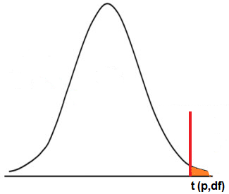
Right-sided t-distibution
Right-sided T-distribution table
| df/p | 0.40 | 0.25 | 0.10 | 0.05 | 0.025 | 0.01 | 0.005 | 0.0005 |
| 1 | 0.324920 | 1.000000 | 3.077684 | 6.313752 | 12.70620 | 31.82052 | 63.65674 | 636.6192 |
| 2 | 0.288675 | 0.816497 | 1.885618 | 2.919986 | 4.30265 | 6.96456 | 9.92484 | 31.5991 |
| 3 | 0.276671 | 0.764892 | 1.637744 | 2.353363 | 3.18245 | 4.54070 | 5.84091 | 12.9240 |
| 4 | 0.270722 | 0.740697 | 1.533206 | 2.131847 | 2.77645 | 3.74695 | 4.60409 | 8.6103 |
| 5 | 0.267181 | 0.726687 | 1.475884 | 2.015048 | 2.57058 | 3.36493 | 4.03214 | 6.8688 |
| 6 | 0.264835 | 0.717558 | 1.439756 | 1.943180 | 2.44691 | 3.14267 | 3.70743 | 5.9588 |
| 7 | 0.263167 | 0.711142 | 1.414924 | 1.894579 | 2.36462 | 2.99795 | 3.49948 | 5.4079 |
| 8 | 0.261921 | 0.706387 | 1.396815 | 1.859548 | 2.30600 | 2.89646 | 3.35539 | 5.0413 |
| 9 | 0.260955 | 0.702722 | 1.383029 | 1.833113 | 2.26216 | 2.82144 | 3.24984 | 4.7809 |
| 10 | 0.260185 | 0.699812 | 1.372184 | 1.812461 | 2.22814 | 2.76377 | 3.16927 | 4.5869 |
| 11 | 0.259556 | 0.697445 | 1.363430 | 1.795885 | 2.20099 | 2.71808 | 3.10581 | 4.4370 |
| 12 | 0.259033 | 0.695483 | 1.356217 | 1.782288 | 2.17881 | 2.68100 | 3.05454 | 4.3178 |
| 13 | 0.258591 | 0.693829 | 1.350171 | 1.770933 | 2.16037 | 2.65031 | 3.01228 | 4.2208 |
| 14 | 0.258213 | 0.692417 | 1.345030 | 1.761310 | 2.14479 | 2.62449 | 2.97684 | 4.1405 |
| 15 | 0.257885 | 0.691197 | 1.340606 | 1.753050 | 2.13145 | 2.60248 | 2.94671 | 4.0728 |
| 16 | 0.257599 | 0.690132 | 1.336757 | 1.745884 | 2.11991 | 2.58349 | 2.92078 | 4.0150 |
| 17 | 0.257347 | 0.689195 | 1.333379 | 1.739607 | 2.10982 | 2.56693 | 2.89823 | 3.9651 |
| 18 | 0.257123 | 0.688364 | 1.330391 | 1.734064 | 2.10092 | 2.55238 | 2.87844 | 3.9216 |
| 19 | 0.256923 | 0.687621 | 1.327728 | 1.729133 | 2.09302 | 2.53948 | 2.86093 | 3.8834 |
| 20 | 0.256743 | 0.686954 | 1.325341 | 1.724718 | 2.08596 | 2.52798 | 2.84534 | 3.8495 |
| 21 | 0.256580 | 0.686352 | 1.323188 | 1.720743 | 2.07961 | 2.51765 | 2.83136 | 3.8193 |
| 22 | 0.256432 | 0.685805 | 1.321237 | 1.717144 | 2.07387 | 2.50832 | 2.81876 | 3.7921 |
| 23 | 0.256297 | 0.685306 | 1.319460 | 1.713872 | 2.06866 | 2.49987 | 2.80734 | 3.7676 |
| 24 | 0.256173 | 0.684850 | 1.317836 | 1.710882 | 2.06390 | 2.49216 | 2.79694 | 3.7454 |
| 25 | 0.256060 | 0.684430 | 1.316345 | 1.708141 | 2.05954 | 2.48511 | 2.78744 | 3.7251 |
| 26 | 0.255955 | 0.684043 | 1.314972 | 1.705618 | 2.05553 | 2.47863 | 2.77871 | 3.7066 |
| 27 | 0.255858 | 0.683685 | 1.313703 | 1.703288 | 2.05183 | 2.47266 | 2.77068 | 3.6896 |
| 28 | 0.255768 | 0.683353 | 1.312527 | 1.701131 | 2.04841 | 2.46714 | 2.76326 | 3.6739 |
| 29 | 0.255684 | 0.683044 | 1.311434 | 1.699127 | 2.04523 | 2.46202 | 2.75639 | 3.6594 |
| 30 | 0.255605 | 0.682756 | 1.310415 | 1.697261 | 2.04227 | 2.45726 | 2.75000 | 3.6460 |
| ∞ | 0.253347 | 0.674490 | 1.281552 | 1.644854 | 1.95996 | 2.32635 | 2.57583 | 3.2905 |
To see this table above as an image file, see the following link: T-distribution table.
Many different distributions exist in statistics, and a commonly used distribution is the t-distribution.
T-distributions are commonly used to find the t-value for a given data set based on the sample size of the data set and the significance level. This t-value can then be used for various statistics settings, including confidence intervals and hypothesis tests.
As background, the normal distribution is the classic and well-known bell-shaped distribution. It is centered around the mean of the data set and has an area of 1 underneath it.
The t-distribution is similar to the normal distribution in that it has a bell curve shape and has an area of 1 underneath it. Like the normal standard distribution, it is centered around the mean, but its standard deviation is proportionally larger compared to the (normal) Z-distribution. So the t-distribution is more stretched out than the Z-distribution.
As with Z-distributions, there is an entire family of different t-distributions. Each different family of t-distribution is determined by the degrees of freedom of the data set. The degrees of freedom (df) of the data set is determined by the sample size. The degrees of freedom (df) is calculated by the formula, df= n-1. So for example, if the sample size is 15, the degrees of freedom will be, df= (n-1)= (15-1)= 14.
Smaller sample sizes have flatter, more stretched out t-distributions than larger sample sizes. As these sample sizes get larger, the t-distributions are less stretched and are taller, approaching the values from the normal standard distribution. The point at which the t-distribution is like the z-distribution is around the point where the degrees of freedom is 30.
So on the t-distribution chart, the row data is the degrees of freedom, which goes from 1 to 30 and then has a row of ∞, where the values are pretty much in line with the Z-distribution.
The columns of the t-distribution show the significance level. As you go from left to right, the significance level becomes more and more accurate. Using the t-distribution chart above, to the right is a significance level of 0.40. This is a confidence level of 60%. The next column is a signficance level of 0.25 (or 75% confidence level). The next column is 0.10 (or 90% confidence level). The next column is 0.05 (or 95% confidence level). The next column is 0.025 (or 97.5%). The next column is 0.01 (or a confidence level of 99%). The next column is 0.005 (or a confidence level of 99.5%). The next column is 0.0005 (or a confidence level of 99.95%).
So, to get the t-value for a certain data set, all we have to know is the degrees of freedom, the significance level, and the hypothesis testing method (one-tail or two-tail).
As an example, let's say we have the following data set group: a sample size of 20, a significance level of 0.10, and one-tail (right-tail) hypothesis testing? What is the t-value?
So doing the math, the sample size is 20, so the degrees of freedom is, df= (n-1)= (20-1)= 19. Looking up the t-value for a df=19 and α= 0.10, we get a t-value of 1.327728.
For two-tail hypothesis testing, this value would be different. This is because two-tail hypothesis testing has 2 sides, left tail and right tail.
This is shown in the diagram below.
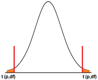
Therefore, with the same example data as above, if we are using two-tail hypothesis testing and we are working with the same significance level of 0.10, our significance level is really 0.05 (since 0.10/2= 0.05). The significance level at the left tail will be 0.05 and the significance level at the right tail will be 0.05. These two added together gives 0.10.
So when you are doing two-tail hypothesis testing with the t-distribution, which you may use if the sample size is below 30 for a data set, then you want to take the significance level and divide it by 2. It is this divided number that gets used as the actual significance level from the t-distribution table when looking up the t-value. This is because each tail of the t-distribution takes half of the significance level each.
So this is a break of the t-distribution table in statistics. ±1 standard deviation from the mean represents 68% of the data set. ±2 standard deviations from the mean represents 95% of the data set. ±3 standard deviations from the mean represents 99.8% of the data set.
Related Resources